Disclaimer: The current post expresses the personal opinion of the author, which may or may not coincide with the opinion of the WHO experts, governmental workers, health care professionals, or other involved institutions. Please check the official web site of the World Health Organisation for the most recent updates on the situation and professional advice.
In this post, we show how to fit the often-mentioned ‘logistic curve’ to COVID-19 cases across various countries using a couple of econometric techniques, and how to compute scenario forecasts.
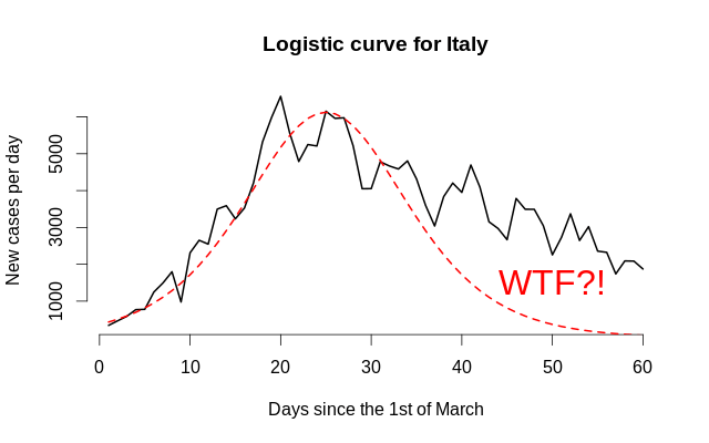
There is one question everyone is asking in Russia: ‘When will our country hit the peak?’ This is a tricky question since the word ‘peak’ usually means ‘the day with the most new cases’ and has little to nothing to do with policy implications. The more general question usually sounds like ‘how will the dynamics look in 2 months’. Many articles—even scientific ones—seem to be talking about some ephemeral ‘logistic curve’. However, there is one problem: climbing in is not the same as climbing out, so the dynamics before and after the peak might vary. Tell me, do these two objects look similar?
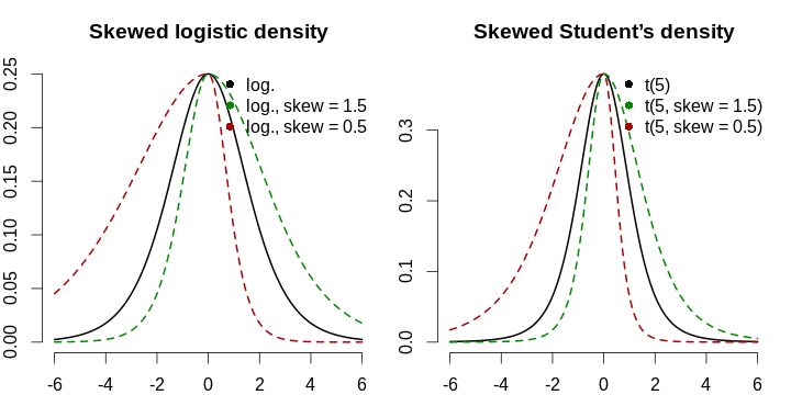
This is why asymmetry must be modelled explicitly. We are going to adopt an approach due to Fernández & Steel (1998), where they generalise symmetrical probability density functions to incorporate the skewness parameter, namely stretching the left part and shrinking the right part by the same factor, and then, normalising to match the first two moments of the original distribution. For the sake of interpretability, we are not going to match the moments since we are not modelling densities; we are just taking the logistic curve, and shifting, scaling, and skewing it in order to match the observed data. Besides that, the logistic curve has exponentially decaying tails, which might not be too realistic due to the commonplace complacency: people think that when there are 10–15 new cases per day, it is over, and begin communicating too closely, and it becomes their (and eveyone’s) undoing. Modelling of tail heaviness (as with Student’s t distribution) could also be an option, but there might be not too many observations to reliably estimate this parameter. The formula for the new-cases-per-day logistic curve will therefore follow the form: \[ g(x; \mu, \sigma, s, h) \mathrel{\stackrel{\text{def}}{=}} \begin{cases} h \cdot f \left( \frac{x - \mu}{\sigma \cdot s} \right), & \frac{x - \mu}{\sigma} > 0, \\ h \cdot f \left( \frac{s(x - \mu)}{\sigma} \right), & \frac{x - \mu}{\sigma} \le 0. \end{cases} \] Here, \(\mu\) is the mode (peak of the function), \(\sigma\) is the spread, \(s\) is the asymmetry coefficient that takes values from \((0, +\infty)\) and shows the relative heaviness of the right tail (\(s > 1\) implies a longer right tail), and finally, \(h\) corresponds to vertical scaling (the number of cases per country matters, so the absolute scale should be inferred from the data, too). Remember that f can be any symmetrical function—here, we are using symmetrical-density-like ones for convenience. Remember that we want a quick answer!
First of all, we download the March and April data from Wikipedia pages titled ‘2020 coronavirus pandemic in X’. We shall focus our attention on Spain, Germany, Italy, Luxembourg, Sweden, Czech Republic, Turkey, and Russia. You will find the data in the table below; please note that these data are as of the 1st of May, 2020, and are subject to change due to methodology updates or new reports.
| Date | spa | ger | ita | lux | swe | cze | tur | rus |
| 2020-03-01 | 85 | 117 | 1,694 | 0 | 7 | 3 | 0 | 0 |
| 2020-03-02 | 121 | 150 | 2,036 | 0 | 7 | 3 | 0 | 3 |
| 2020-03-03 | 166 | 188 | 2,502 | 0 | 11 | 5 | 0 | 3 |
| 2020-03-04 | 228 | 240 | 3,089 | 0 | 16 | 5 | 0 | 3 |
| 2020-03-05 | 282 | 349 | 3,858 | 2 | 17 | 8 | 0 | 4 |
| 2020-03-06 | 401 | 534 | 4,636 | 3 | 22 | 19 | 0 | 10 |
| 2020-03-07 | 525 | 684 | 5,883 | 4 | 29 | 26 | 0 | 14 |
| 2020-03-08 | 674 | 847 | 7,375 | 5 | 38 | 32 | 0 | 17 |
| 2020-03-09 | 1,231 | 1,112 | 9,172 | 5 | 54 | 38 | 0 | 20 |
| 2020-03-10 | 1,695 | 1,460 | 10,149 | 7 | 108 | 63 | 0 | 20 |
| 2020-03-11 | 2,277 | 1,884 | 12,462 | 7 | 181 | 94 | 1 | 28 |
| 2020-03-12 | 3,146 | 2,369 | 15,113 | 26 | 238 | 116 | 1 | 34 |
| 2020-03-13 | 5,232 | 3,062 | 17,660 | 34 | 266 | 141 | 5 | 45 |
| 2020-03-14 | 6,391 | 3,795 | 21,157 | 51 | 292 | 189 | 6 | 59 |
| 2020-03-15 | 7,988 | 4,838 | 24,747 | 77 | 339 | 298 | 18 | 63 |
| 2020-03-16 | 9,942 | 6,012 | 27,980 | 81 | 384 | 383 | 47 | 93 |
| 2020-03-17 | 11,826 | 7,156 | 31,506 | 140 | 425 | 450 | 98 | 114 |
| 2020-03-18 | 14,769 | 8,198 | 35,713 | 203 | 511 | 560 | 191 | 147 |
| 2020-03-19 | 18,077 | 10,999 | 41,035 | 335 | 603 | 765 | 359 | 199 |
| 2020-03-20 | 21,571 | 13,957 | 47,021 | 484 | 685 | 889 | 670 | 253 |
| 2020-03-21 | 25,496 | 16,662 | 53,578 | 670 | 767 | 1,047 | 947 | 306 |
| 2020-03-22 | 29,909 | 18,610 | 59,138 | 798 | 845 | 1,161 | 1,236 | 367 |
| 2020-03-23 | 35,480 | 22,672 | 63,927 | 875 | 927 | 1,287 | 1,529 | 438 |
| 2020-03-24 | 42,058 | 27,436 | 69,176 | 1,099 | 1,027 | 1,472 | 1,872 | 495 |
| 2020-03-25 | 50,105 | 31,554 | 74,386 | 1,333 | 1,125 | 1,763 | 2,433 | 658 |
| 2020-03-26 | 57,786 | 36,508 | 80,539 | 1,453 | 1,228 | 2,022 | 3,629 | 840 |
| 2020-03-27 | 65,719 | 42,288 | 86,498 | 1,605 | 1,317 | 2,395 | 5,698 | 1,036 |
| 2020-03-28 | 73,232 | 48,582 | 92,472 | 1,831 | 1,392 | 2,657 | 7,402 | 1,264 |
| 2020-03-29 | 80,110 | 52,547 | 97,689 | 1,950 | 1,450 | 2,817 | 9,217 | 1,534 |
| 2020-03-30 | 87,956 | 57,298 | 101,739 | 1,988 | 1,566 | 3,001 | 10,827 | 1,836 |
| 2020-03-31 | 95,923 | 61,913 | 105,792 | 2,178 | 1,683 | 3,308 | 13,531 | 2,337 |
| 2020-04-01 | 104,118 | 67,366 | 110,574 | 2,319 | 1,828 | 3,589 | 15,679 | 2,777 |
| 2020-04-02 | 112,065 | 73,522 | 115,242 | 2,487 | 1,982 | 3,858 | 18,135 | 3,548 |
| 2020-04-03 | 119,199 | 79,696 | 119,827 | 2,612 | 2,179 | 4,190 | 20,921 | 4,149 |
| 2020-04-04 | 126,168 | 85,778 | 124,632 | 2,729 | 2,253 | 4,472 | 23,934 | 4,731 |
| 2020-04-05 | 131,646 | 91,714 | 128,948 | 2,804 | 2,359 | 4,587 | 27,069 | 5,389 |
| 2020-04-06 | 136,675 | 95,391 | 132,547 | 2,843 | 2,566 | 4,822 | 30,217 | 6,343 |
| 2020-04-07 | 141,942 | 99,225 | 135,586 | 2,970 | 2,763 | 5,017 | 34,109 | 7,497 |
| 2020-04-08 | 148,220 | 103,228 | 139,422 | 3,034 | 2,890 | 5,312 | 38,226 | 8,672 |
| 2020-04-09 | 153,222 | 108,202 | 143,626 | 3,115 | 3,036 | 5,569 | 42,282 | 10,131 |
| 2020-04-10 | 158,273 | 113,525 | 147,577 | 3,223 | 3,100 | 5,732 | 47,029 | 11,917 |
| 2020-04-11 | 163,027 | 117,658 | 152,271 | 3,270 | 3,175 | 5,902 | 52,167 | 13,584 |
| 2020-04-12 | 166,831 | 120,479 | 156,363 | 3,281 | 3,254 | 5,991 | 56,956 | 15,770 |
| 2020-04-13 | 170,099 | 123,016 | 159,516 | 3,292 | 3,369 | 6,059 | 61,049 | 18,328 |
| 2020-04-14 | 174,060 | 125,098 | 162,488 | 3,307 | 3,539 | 6,141 | 65,111 | 21,102 |
| 2020-04-15 | 180,659 | 127,584 | 165,155 | 3,373 | 3,665 | 6,301 | 69,392 | 24,490 |
| 2020-04-16 | 184,948 | 130,450 | 168,941 | 3,444 | 3,785 | 6,433 | 74,193 | 27,938 |
| 2020-04-17 | 190,839 | 133,830 | 172,434 | 3,480 | 3,909 | 6,549 | 78,546 | 32,008 |
| 2020-04-18 | 194,416 | 137,439 | 175,925 | 3,537 | 3,964 | 6,654 | 82,329 | 36,793 |
| 2020-04-19 | 198,674 | 139,897 | 178,972 | 3,550 | 4,027 | 6,746 | 86,306 | 42,853 |
| 2020-04-20 | 200,210 | 141,672 | 181,228 | 3,558 | 4,173 | 6,900 | 90,980 | 47,121 |
| 2020-04-21 | 204,178 | 143,457 | 183,957 | 3,618 | 4,284 | 7,033 | 95,591 | 52,763 |
| 2020-04-22 | 208,389 | 145,694 | 187,327 | 3,654 | 4,406 | 7,132 | 98,674 | 57,999 |
| 2020-04-23 | 213,024 | 148,046 | 189,973 | 3,665 | 4,515 | 7,187 | 101,790 | 62,773 |
| 2020-04-24 | 219,764 | 150,383 | 192,994 | 3,695 | 4,610 | 7,273 | 104,912 | 68,622 |
| 2020-04-25 | 223,759 | 152,438 | 195,351 | 3,711 | 4,686 | 7,352 | 107,773 | 74,588 |
| 2020-04-26 | 226,629 | 154,175 | 197,675 | 3,723 | 4,756 | 7,404 | 110,130 | 80,949 |
| 2020-04-27 | 229,422 | 155,193 | 199,414 | 3,729 | 4,884 | 7,445 | 112,261 | 87,147 |
| 2020-04-28 | 232,128 | 156,337 | 201,505 | 3,741 | 4,980 | 7,504 | 114,653 | 93,558 |
| 2020-04-29 | 236,899 | 157,641 | 203,591 | 3,769 | 5,040 | 7,579 | 117,589 | 99,399 |
| 2020-04-30 | 239,369 | 159,119 | 205,463 | 3,784 | 5,051 | 7,682 | 120,204 | 106,498 |
Secondly, we have to choose the estimation method. Basically, for every country, we have pairs of observations \((1, Y_1), (2, Y_2), \ldots, (61, Y_{61})\), and the functional form is assumed to be known up to 4 (logistic) or 5 (Student) parameters. The most obvious way of estimation is minimising some statistic based on the discrepancies between the real data and the model predictions, the easiest case being squared errors and the sum thereof. However, often in practice more robust penalty functions are used, and sometimes, more robust statistics, so here, we shall also try minimising the sum of absolute deviations (like in a quantile non-linear regression) and the median of squared errors (like in a Least-Median-of-Squares regression due to Rousseeuw). We shall be minimising these 3 criteria. Note that the last one is not smooth in parameters, so there might be a continuum of parameter values yielding the global minimum of the criterion. \[ C_1 = \frac{1}{n} \sum_{t=1}^T (Y_t - g(t; \theta))^2, \quad C_2 = \frac{1}{n} \sum_{t=1}^T |Y_t - g(t; \theta)|, \quad C_3 = \mathrm{median}[(Y_t - g(t; \theta))^2] \] Thirdly, since we are modelling parametric curves with four intuitive parameters, we pick some ballpark estimates in order to roughly match the dynamics. The criterion function is highly non-linear in parameters, so we begin by manually fiddling with parameters for each of our countries, and then, constructing a rather generous hypercube around it and trying a stochastic optimisation routine to pick the candidate for the best solution. We further refine it with constrained Nelder—Mead optimiser.
We implement the general curve via a custom function that depends on the data points (days elapsed from the 1st of March), distribution type (we consider logistic and Student, but other ones are possible), and finally, distribution parameters (a vector of length 4 or 5: mean, scale, skewness, height multiplier, and for Student’s t distribution, the number of degrees of freedom).
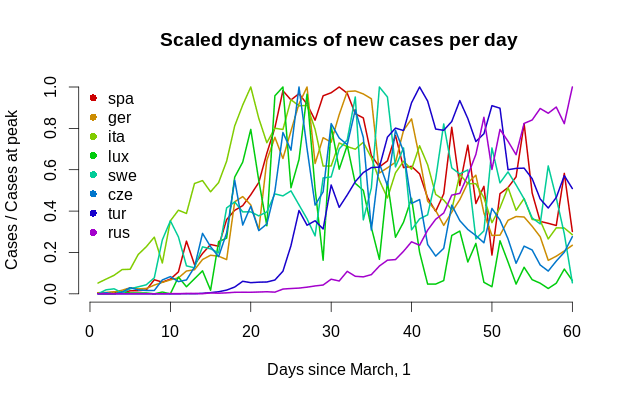
Remember, we do not refer to this function as to density since we do not know the real scale; it is just a curve, and its unit of measurement is, well, people, so it measures the number of cases. This is how all dynamics look in one graph.
Now, it is time to choose reasonable starting values for the optimiser because they belong to various scales. For numerical stability, especially for gradient-based methods, it is reasonable to have all parameters of the same order of magnitude (say, via rescaling), and it seems like the vertical scale parameter is in the range of tens of thousands, so we divide it by 10,000. For every country, we eyeballed the parameters \((\tilde \mu, \tilde\sigma, \tilde s, \tilde h\ [, \widetilde{df}])\), and then set the following ranges for stochastic search: \((\tilde\mu/2, \tilde\sigma/3, \tilde s/3, \tilde h / 4\ [, 0.1])\) to \((1.5\tilde\mu, 3\tilde\sigma, 3\tilde s, 3\tilde h\ [, 50])\).
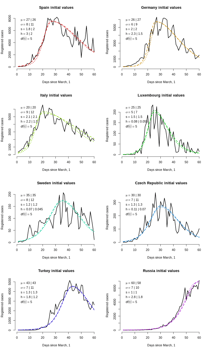
For optimisation, we are using the hydroPSO library with its excellent parallel capabilities and many tweaks. Since high-dimensional spaces are getting sparser than one can imagine, for a more thorough sweep, we are using a population of size 400 or 600. Convergence is quite quick for the logistic model, and somewhat slower for the Student’s one, so we use 50–100 iterations for the former and 75–125 iterations for the latter (this is a rough first-step preëstimation anyway). One iteration took 0.25–0.5 seconds, so estimating all models took 8 ⋅ (50 + 75 + 100 + 75 + 100 + 125) ⋅ 0.35 ≈ 1500 seconds, or roughly half an hour—a small price to pay for robustness against multiple local optima.
You would think that estimation can continue without a hindrance... right? Wrong!
There is one cloud on the horizon: so far, there has been no peak in Russia... yet! This open a whole new can of worms: strictly speaking, the skewness parameter and the scale parameter are not identified because we observe only the left side of the distribution: one can multiply the skewness parameter by 2 and the scale parameter by 2, and get the same left tail. Relying on the rightmost end of the data is a dangerous affair in this case. It is well-known that estimation of the truncated normal parameters when the mean is outside the truncation range is very unreliable; in our situation, the peak is also outside the range, which makes our problem even worse. This means that for the purposes of estimation, the skewness parameter must be set to that of other countries, so only scale will be estimated. E. g. if Russia were to follow the right-tail decay model of Luxembourg, what would the total number of cases be? In other words, we can make scenario forecasts: Turkish scenario, Italian scenario, average scenario.
The second-step maximisation from the candidate solution was done in a blink of an eye, and the estimates themselves did not change much. However, the results were more volatile for Sweden, one model returned strange results for Turkey, and, as expected, the results for Russia were quite strange—because we have not applied the magic fix yet.
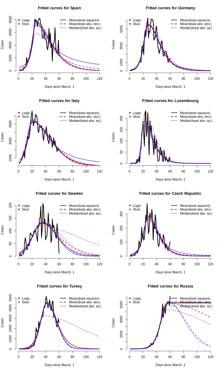
Now it is obvious that there is no clear winner among the models, and both logistic and Student’s fit yield similar fits. For the sake of parsimony, we restrict our analysis to logistic fits only and forget about tail heaviness estimation.
Besides that, in this estimation, we are not worrying about statistical inference. Of course, for the NLS estimator, one can compute robust standard errors, but for these data, it is non-trivial to do so for the two other estimators, and the data are dependent, so there is no obvious solution. Remember, we are keeping it simple here.
Now comes the part everyone is eagerly waiting for: how many cases are expected to occur in the upcoming months? Or, say, on which date are we expecting less than one person to be infected? Or even better, when are we expecting less than 1 case in two weeks (that is, 1/14 cases per day), and what will be the toll up until that date—so we can call it the end of the pandemic? For this, we can invoke a very simple computation: increase the time frame to the right by as much as we want, and just find the points where that curve takes values 1 or 1/14. The total expected number of cases will be the cumulative sum up until that date.
Now, we use the logistic models to forecast the number of cases in each country until the day less than 1 case or less than 1/14 cases per day. For every country, we pick the best model (out of three logistic ones) as the one that predicted the closest number of total cases up to the last date (i. e. the best in-sample fit).
| Real cases by April, 30 | Mean least squares | Mean abs. dev. | Median least sq. | |
| Spain | 239,369 | 237,304 | 242,555 | 203,910 |
| Germany | 159,119 | 158,465 | 164,505 | 183,371 |
| Italy | 205,463 | 203,246 | 204,339 | 212,175 |
| Luxembourg | 3,784 | 3,749 | 4,108 | 5,147 |
| Sweden | 5,051 | 5,076 | 5,046 | 5,160 |
| Czech Republic | 7,682 | 7,646 | 7,710 | 8,033 |
| Turkey | 120,204 | 121,944 | 116,104 | 102,600 |
| Cases by April, 30 | Days from March, 1 till 1 new case/day | Days from March, 1 till 1 new case/14 days | Cases till 1 new case/day | Cases till 1 new case/14 days |
| 239,369 | 189 | 231 | 282,401 | 282,415 |
| 159,119 | 142 | 172 | 171,369 | 171,379 |
| 205,463 | 201 | 249 | 241,977 | 241,993 |
| 3,784 | 83 | 109 | 3,838 | 3,847 |
| 5,051 | 148 | 196 | 6,752 | 6,768 |
| 7,682 | 95 | 120 | 8,029 | 8,037 |
| 120,204 | 140 | 166 | 145,922 | 145,930 |
| Peak (μ) | Horiz. scale (σ) | Skewness (s) | Vert. scale (h) | |
| Spain | 25.383 | 7.859 | 2.026 | 2.854 |
| Germany | 27.533 | 7.050 | 1.612 | 2.180 |
| Italy | 20.519 | 9.619 | 1.881 | 2.103 |
| Luxembourg | 20.131 | 3.999 | 2.410 | 0.068 |
| Sweden | 32.858 | 12.033 | 1.519 | 0.052 |
| Czech Republic | 27.818 | 6.764 | 1.400 | 0.113 |
| Turkey | 41.888 | 7.754 | 1.277 | 1.829 |
But... wait! What about Russia?
We have 7 countries and 7 different scenarios. In terms of parameters, these scenarios are described by the peak day (\(\mu\)), steepness of the curve (\(\sigma\)), asymmetry (\(s\)), overall scale (\(h\)), and for Russia, we cannot know the degree of asymmetry. Compare these two plots.
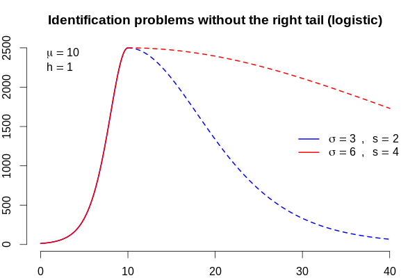
For the same left tail, we get the red right tail that is 4 times heavier than the blue one. This has huge implication for the forecasts as well: the blue curve describes a pandemic that decreases to less than 1 new case per day in 66 days with 37,469 cases, and the red one will take a whopping 232 days with 127,451 infections! This means that the initial values for Russia must be tweaked according to all 7 scenarios for other countries.
After we re-estimate the logistic model for Russia with skewness fixed to 1 (least absolute deviations yielded a slightly better total number of cases, with relative error slightly less than 1%), we can multiply both the scale \(\sigma\) and the skewness \(s\) by other countries’ skewnesses, compute the two sacred days (less than 1 case per 1 day or per 14 days), and obtain the total number of cases.
The estimates for Russia are: \(\hat\mu = 56.1\), \(\hat\sigma / s = 6.33\), \(\hat h = 2.49\). This means that, despite the lack of clear peak by day 61, it must have occurred on day 56, just before the end of data collection.
| Days till 1 new case/day | Days till 1 new case/14 days | Cases till 1 new case/day | Cases till 1 new case/14 days | |
| Spain scenario | 320 | 388 | 402,422 | 402,445 |
| Germany scenario | 223 | 267 | 283,730 | 283,745 |
| Italy scenario | 284 | 343 | 357,887 | 357,907 |
| Luxembourg scenario | 429 | 526 | 536,540 | 536,573 |
| Sweden scenario | 205 | 243 | 260,712 | 260,724 |
| Czech Republic scenario | 182 | 215 | 233,328 | 233,339 |
| Turkey scenario | 161 | 188 | 207,443 | 207,452 |
| Average scenario (s = 1.73) | 249 | 299 | 315,371 | 315,387 |
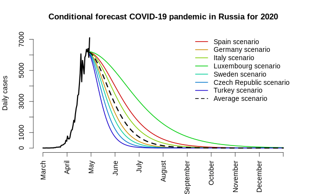
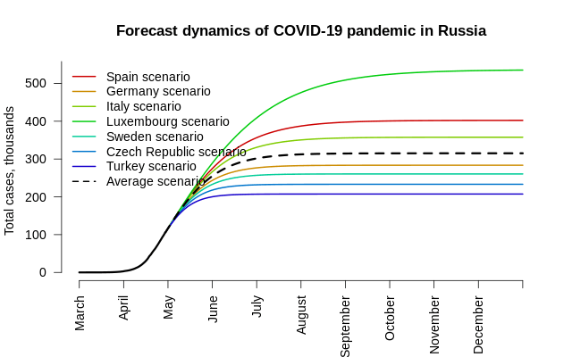
Before we jump to the conclustion, there are several ‘buts’ worth mentionings:
- Inferring the shift of the curve (\(\hat\mu\)) from the left part is very unreliable, so there is a huge confidence band around that estimate. How huge? It is up to the dear reader to compute the standard errors, but no one should even assume normality of the estimator since it is well known that the behaviour of estimators on the boundary of the parameter space is far from asymptotically normal (cf. the failure of maximal likelihood for estimation of extreme order statistics).
- The ‘peak’, although defined as the maximum number of cases, in our estimation, corresponds to th peak of the smoother underlying curve, even if individual observations can jump above or below, assuming, among others, that the error is mean zero. If there is systematic under-reporting because there are not enough tests available and the real numbers are higher, this overly simplistic model cannot learn anything useful from the data, and other, more sophisticated methods must be used.
- There are many asymptomatic cases that are not registered anywhere that are making up the underwater part of the iceberg, so if that iceberg of unobservedness were to be raised entirely above water, the peak would shift to the right.
- The reported daily numbers depend heavily on testing tactics, good weather (this is not ‘sunspot economics’ envisioned by Jevons, this correlates with the number of people gathering outside), presidental speeches, and other hidden variables.
All these caveates hint at the fact that what we obtained is an under-estimate of the real peak, but dealing with the problems outlined above required better spatial data, more information about the population density, geographical distribution—a real job for real epidemilogists.
We conclude the following (if Russia follows the dynamics of some European countries and if one blisfully ignores the caveats above):
- The peak is most likely to have already occurred at the very end of April, 2020;
- The total number of infected people will be between 200 and 500 hundred thousand Russian citizens;
- Under the assumption of average asymmetrical European scenario (where the decrease of cases per day after the peak is roughly 3 times slower than the growth prior to reaching the peak), the total number of cases is estimated to be 315 thousand;
- In early November, the number of new cases per day will become less than 1, and by the end of December, the number, there will be fewer than 1 case per 2 weeks.
Only time will tell how accurate these quick estimates are, so you are encouraged to redo the estimation on new data (maybe with more countries) and update the forecasts.
Copy the table above into R under the name ds (data frame) and use the code below to replicate these results.
library(hydroPSO)
library(stargazer)

cs <- c("spa", "ger", "ita", "lux", "swe", "cze", "tur", "rus")
csn <- c("Spain", "Germany", "Italy", "Luxembourg", "Sweden", "Czech Republic", "Turkey", "Russia")
# Uncomment this for Cyrillic names
# csn <- c("Испания", "Германия", "Италия", "Люксембург", "Швеция", "Чехия", "Турция", "Россия")
d <- lapply(cs, function(x) readLines(paste0(x, ".fsf")))

clean <- function(x) {
  x <- gsub("\\s+", " ", x)
  x <- gsub(" $", "", x)
  x <- gsub(",", "", x)
  x <- gsub("\\([^)]+\\)", "", x)
  x
}

d <- lapply(d, function(x) strsplit(clean(x), " "))
d <- lapply(d, function(y) lapply(y, function(x) if (length(x) == 2) x else x[1:2]) )
d <- lapply(d, function(x) as.data.frame(do.call(rbind, x), stringsAsFactors = FALSE))
d <- lapply(d, function(x) {colnames(x) <- c("Date", "Cases"); x})

ds <- Reduce(
  function(x, y) merge(x, y, all = TRUE, by = "Date"),
  d
)
colnames(ds) <- c("Date", cs)

for (i in 2:ncol(ds)) {
  ds[, i] <- as.numeric(ds[, i])
  if (is.na(ds[1, i])) {
    nm <- which(is.finite(ds[, i]))[1]
    ds[1:(nm-1), i] <- 0
  }
}

ds <- ds[1:61, ]

stargazer(ds, type = "html", summary = FALSE, out = "blog.html", rownames = FALSE)

mycurve <- function(x, distrib, pars) {
  pars[4] <- pars[4] * 1e4
  xstd <- (x - pars[1]) / pars[2]
  f <- switch(distrib,
              logistic = ifelse(xstd > 0, dlogis(xstd/pars[3]), dlogis(xstd*pars[3])) * pars[4],
              student = ifelse(xstd > 0, dt(xstd/pars[3], df = pars[5]), dt(xstd*pars[3], df = pars[5])) * pars[4]
  )
  return(f)
}

png("plot1-logistic-curve-coronavirus-italy.png", 640, 400, type = "cairo", pointsize = 16)
plot(diff(ds$ita), type = "l", xlab = "Days since the 1st of March", ylab = "New cases per day",
     bty = "n", lwd = 2, main = "Logistic curve for Italy")
lines(1:60, mycurve(1:60, "logistic", c(25, 6, 1, 2.45)), col = "red", lty = 2, lwd = 2)
text(50, 1500, "WTF?!", col = "red", cex = 2)
dev.off()

mycols <- c("#000000", "#008800", "#AA0000")

png("plot2-density-logistic-curve-for-corona-virus-flattening.png", 720, 360, pointsize = 16)
par(mar = c(2, 2, 3, 1), mfrow = c(1, 2))
curve(dlogis(x), -6, 6, n = 1001, main = "Skewed logistic density", bty = "n",
      lwd = 2, ylim = c(0, dlogis(0)), ylab = "", xlab = "")
curve(mycurve(x, "logistic", c(0, 1, 1.5, 1e-4)), -6, 6, n = 1001, add = TRUE,
      col = mycols[2], lwd = 2, lty = 2)
curve(mycurve(x, "logistic", c(0, 1, 0.5, 1e-4)), -6, 6, n = 1001, add = TRUE,
      col = mycols[3], lwd = 2, lty = 2)
legend("topright", c("log.", "log., skew = 1.5", "log., skew = 0.5"), col = mycols, pch = 16, bty = "n")

curve(dt(x, 5), -6, 6, n = 1001, main = "Skewed Student’s density", bty = "n",
      lwd = 2, ylim = c(0, dt(0, 5)))
curve(mycurve(x, "student", c(0, 1, 1.5, 1e-4, 5)), -6, 6, n = 1001, add = TRUE,
      col = mycols[2], lwd = 2, lty = 2)
curve(mycurve(x, "student", c(0, 1, 0.5, 1e-4, 5)), -6, 6, n = 1001, add = TRUE,
      col = mycols[3], lwd = 2, lty = 2)
legend("topright", c("t(5)", "t(5, skew = 1.5)", "t(5, skew = 0.5)"), col = mycols, pch = 16, bty = "n")
dev.off()

ds[, (length(cs)+2):(length(cs)*2+1)] <- sapply(ds[, 2:(length(cs)+1)], function(x) diff(c(NA, x)))
colnames(ds)[(length(cs)+2):(length(cs)*2+1)] <- paste0("d", cs)
ds <- ds[2:nrow(ds), ]

mycols <- rainbow(length(cs), end = 0.8, v = 0.8)
png("plot3-new-covid-19-cases-as-a-fraction-of-maximum.png", 640, 400, pointsize = 16)
plot(NULL, NULL, xlim = c(1, nrow(ds)), ylim = c(0, 1), xlab = "Days since March, 1",
     ylab = "Cases / Cases at peak", bty = "n", main = "Scaled dynamics of new cases per day")
for (i in (length(cs)+2):(length(cs)*2+1)) lines(ds[, i] / max(ds[, i]),
                                                 type = "l", lwd = 2, col = mycols[i - length(cs) - 1])
legend("topleft", cs, pch = 16, col = mycols, bty = "n")
dev.off()

start.pars <- list(list(c(27, 8, 1.8, 3), c(26, 11, 2, 2, 5)), # Spain
                   list(c(26, 6, 2, 2.3), c(27, 9, 2, 1.5, 5)), # Germany
                   list(c(20, 9, 2.1, 2.2), c(20, 12, 2.1, 1.5, 5)), # Italy
                   list(c(25, 5, 1.5, 0.08), c(25, 7, 1.5, 0.055, 5)), # Luxembourg
                   list(c(35, 8, 1.2, 0.07), c(35, 12, 1.2, 0.045, 5)), # Sweden
                   list(c(30, 7, 1.3, 0.11), c(30, 11, 1.3, 0.07, 5)), # Czech,
                   list(c(43, 7, 1.3, 1.8), c(43, 11, 1.3, 1.2, 5)), # Turkey
                   list(c(60, 7, 1, 2.8), c(58, 10, 1, 1.8, 5)) # Russia
                   )
start.pars <- lapply(start.pars, function(x) {names(x) <- c("logistic", "student"); x})

leg <- function(i) {
  c(parse(text = paste0('mu == ', start.pars[[i]][[1]][1], '*" | "*', start.pars[[i]][[2]][1])),
    parse(text = paste0('sigma == ', start.pars[[i]][[1]][2], '*" | "*', start.pars[[i]][[2]][2])),
    parse(text = paste0('s == ', start.pars[[i]][[1]][3], '*" | "*', start.pars[[i]][[2]][3])),
    parse(text = paste0('h == ', start.pars[[i]][[1]][4], '*" | "*', start.pars[[i]][[2]][4])),
    parse(text = paste0('df(t) == ', start.pars[[i]][[2]][5])))
}

png("plot4-initial-values-for-search.png", 720, 1200, pointsize = 16)
par(mfrow = c(4, 2))
for (i in 1:length(cs)) {
  plot(ds[, paste0("d", cs[i])], type = "l", lwd = 2,
       xlab = "Days since March, 1",        ylab = "Registered cases", bty = "n",
       main = paste0(csn[i], " initial values"), ylim = c(0, max(ds[, paste0("d", cs[i])])))
  lines(mycurve(1:nrow(ds), "logistic", start.pars[[i]][[1]]), col = mycols[i], lwd = 2, lty = 2)
  lines(mycurve(1:nrow(ds), "student", start.pars[[i]][[2]]), col = mycols[i], lwd = 2, lty = 3)
  legend("topleft", legend = leg(i), bty = "n")
}
dev.off()

criterion <- function(pars, observed, distrib, fun = function(x) mean(x^2)) {
  theor <- mycurve(x = 1:length(observed), distrib = distrib, pars = pars)
  return(fun(theor - observed))
}

rls <- function(x) sqrt(mean(x^2)) # Root mean least square; root is here for the purposes of comparison
nla <- function(x) mean(abs(x))
nms <- function(x) sqrt(median(x^2)) # Root median of squares
opt.res <- vector("list", length(cs))
for (i in 1:length(cs)) {
  sl <- start.pars[[i]][[1]]
  st <- start.pars[[i]][[2]]
  ll <- start.pars[[i]][[1]] / c(2, 3, 3, 4) # Lower bound for logistic
  ul <- start.pars[[i]][[1]] * c(1.5, 3, 3, 3) # Upper bound for logistic
  lt <- c(start.pars[[i]][[2]][1:4] / c(2, 3, 3, 4), 0.1) # Lower bound for Student
  ut <- c(start.pars[[i]][[2]][1:4] * c(1.5, 3, 3, 3), 50) # Upper bound for Student
  contl1 <- list(npart = 400, REPORT = 1, parallel = "parallel", par.nnodes = 6, maxit = 50, plot = TRUE)
  contl2 <- list(npart = 400, REPORT = 1, parallel = "parallel", par.nnodes = 6, maxit = 75, plot = TRUE)
  contl3 <- list(npart = 400, REPORT = 1, parallel = "parallel", par.nnodes = 6, maxit = 100, plot = TRUE)
  contt1 <- list(npart = 600, REPORT = 1, parallel = "parallel", par.nnodes = 6, maxit = 75, plot = TRUE)
  contt2 <- list(npart = 600, REPORT = 1, parallel = "parallel", par.nnodes = 6, maxit = 100, plot = TRUE)
  contt3 <- list(npart = 600, REPORT = 1, parallel = "parallel", par.nnodes = 6, maxit = 125, plot = TRUE)
  set.seed(1); cat(csn[i], "logistic: least squares\n")
  opt.log.nls <- hydroPSO(par = sl, fn = function(x) criterion(x, ds[, paste0("d", cs[i])], "logistic", rls),
                          lower = ll, upper = ul, control = contl1)
  set.seed(1); cat(csn[i], "logistic: least absolute deviations\n")
  opt.log.nla <- hydroPSO(par = sl, fn = function(x) criterion(x, ds[, paste0("d", cs[i])], "logistic", nla),
                          lower = ll, upper = ul, control = contl2)
  set.seed(1); cat(csn[i], "logistic: median of least squares\n")
  opt.log.nms <- hydroPSO(par = sl, fn = function(x) criterion(x, ds[, paste0("d", cs[i])], "logistic", nms),
                          lower = ll, upper = ul, control = contl3)
  set.seed(1); cat(csn[i], "student: least squares\n")
  opt.t.nls <- hydroPSO(par = st, fn = function(x) criterion(x, ds[, paste0("d", cs[i])], "student", rls),
                        lower = lt, upper = ut, control = contt1)
  set.seed(1); cat(csn[i], "student: least absolute deviations\n")
  opt.t.nla <- hydroPSO(par = st, fn = function(x) criterion(x, ds[, paste0("d", cs[i])], "student", nla),
                        lower = lt, upper = ut, control = contt2)
  set.seed(1); cat(csn[i], "student: median of least squares\n")
  opt.t.nms <- hydroPSO(par = st, fn = function(x) criterion(x, ds[, paste0("d", cs[i])], "student", nms),
                        lower = lt, upper = ut, control = contt3)

  opt.res[[i]] <- list(opt.log.nls, opt.log.nla, opt.log.nms, opt.t.nls, opt.t.nla, opt.t.nms)
  save(opt.res, file = "opt.RData", compress = "xz")
}

ui4 <- diag(4)
ci4 <- c(10, 1, 0.01, 1e-5)
ui5 <- diag(5)
ci5 <- c(10, 1, 0.01, 1e-5, 0.1)

opt.refined <- vector("list", length(cs))
for (i in 1:length(cs)) {
  cat(csn[i], "\n")
  sl1 <- opt.res[[i]][[1]]$par # Replace with start.pars[[i]]$logistic if you did not do the stochastic optimisation
  sl2 <- opt.res[[i]][[2]]$par # Replace with start.pars[[i]]$logistic if you did not do the stochastic optimisation
  sl3 <- opt.res[[i]][[3]]$par # Replace with start.pars[[i]]$logistic if you did not do the stochastic optimisation
  st1 <- opt.res[[i]][[4]]$par # Replace with start.pars[[i]]$student if you did not do the stochastic optimisation
  st2 <- opt.res[[i]][[5]]$par # Replace with start.pars[[i]]$student if you did not do the stochastic optimisation
  st3 <- opt.res[[i]][[6]]$par # Replace with start.pars[[i]]$student if you did not do the stochastic optimisation

  opt.log.nls <- constrOptim(sl1, function(x) criterion(x, ds[, paste0("d", cs[i])], "logistic", rls),
                             grad = NULL, ui = ui4, ci = ci4, outer.iterations = 300)
  opt.log.nla <- constrOptim(sl2, function(x) criterion(x, ds[, paste0("d", cs[i])], "logistic", nla),
                             grad = NULL, ui = ui4, ci = ci4, outer.iterations = 300)
  opt.log.nms <- constrOptim(sl3, function(x) criterion(x, ds[, paste0("d", cs[i])], "logistic", nms),
                             grad = NULL, ui = ui4, ci = ci4, outer.iterations = 300)
  opt.t.nls <- constrOptim(st1, function(x) criterion(x, ds[, paste0("d", cs[i])], "student", rls),
                           grad = NULL, ui = ui5, ci = ci5, outer.iterations = 300)
  opt.t.nla <- constrOptim(st2, function(x) criterion(x, ds[, paste0("d", cs[i])], "student", nla),
                           grad = NULL, ui = ui5, ci = ci5, outer.iterations = 300)
  opt.t.nms <- constrOptim(st2, function(x) criterion(x, ds[, paste0("d", cs[i])], "student", nms),
                           grad = NULL, ui = ui5, ci = ci5, outer.iterations = 300)

  opt.refined[[i]] <- list(opt.log.nls, opt.log.nla, opt.log.nms, opt.t.nls, opt.t.nla, opt.t.nms)
}
save(opt.res, opt.refined, file = "opt.RData", compress = "xz")

xmax <- 120
xinf <- 1000

mycols <- c("#CC0000", "#0000FFCC")
png("plot5-fitted-logistic-curve-total-infected-coronavirus-cases.png", 720, 1200, type = "cairo", pointsize = 16)
par(mfrow = c(4, 2))
for (i in 1:length(cs)) {
  plot(ds[, paste0("d", cs[i])], xlim = c(1, xmax), type = "l", lwd = 3,
       xlab = "Days since March, 1", ylab = "Cases", bty = "n", main = paste0("Fitted curves for ", csn[i]))
  for (j in 1:3) {
    lines(mycurve(1:xmax, distrib = "logistic", pars = opt.refined[[i]][[j]]$par), lwd = 2, lty = j, col = mycols[1])
    lines(mycurve(1:xmax, distrib = "student", pars = opt.refined[[i]][[j + 3]]$par), lwd = 2, lty = j, col = mycols[2])
  }
  legend("topleft", c("Logis.", "Stud."), pch = 16, col = mycols, bty = "n")
  legend("topright", c("Mean(least squares)", "Mean(least abs. dev.)", "Median(least abs. sq.)"),
         lty = 1:3, lwd = 2, bty = "n")
}
dev.off()

res.tab <- vector("list", length(cs))
for (i in 1:length(cs)) {
  cat(csn[i])
  a <- cbind(c(start.pars[[i]]$logistic, NA), c(opt.refined[[i]][[1]]$par, NA),
             c(opt.refined[[i]][[2]]$par, NA), c(opt.refined[[i]][[3]]$par, NA),
             start.pars[[i]]$student, opt.refined[[i]][[4]]$par,
             opt.refined[[i]][[5]]$par, opt.refined[[i]][[6]]$par)
  colnames(a) <- c("Log. init. val.", "Log. LS", "Log. LAD", "Log. LMS",
                   "Stud. init. val.", "Stud. LS", "Stud. LAD", "Stud. LMS")
  row.names(a) <- c("Peak", "Horiz. scale", "Skew", "Vert. scale", "Stud. DoF")
  res.tab[[i]] <- a
  # stargazer(a, out = paste0(csn[i], ".html"), type = "html", summary = FALSE, digits = 2)
}

find.day <- function(cases, distrib, pars) {
  uniroot(function(x) mycurve(x, distrib, pars) - cases,
          lower = pars[1], upper = pars[1] + 180, extendInt = "downX", maxiter = 200, tol = 1e-8)$root
}

get.cases <- function(xmax, distrib, pars) {
  round(sum(mycurve(1:xmax, distrib, pars)))
}

days.to.one <- days.to.tw <- cases.one <- cases.tw <- cases.insample <- matrix(NA, nrow = length(cs), ncol = 6)
best.mod <- best.log <- numeric(length(cs))
for (i in 1:length(cs)) {
  days.to.one[i, ] <- c(sapply(1:3, function(j) find.day(1, "logistic", opt.refined[[i]][[j]]$par)),
                        sapply(4:6, function(j) find.day(1, "student", opt.refined[[i]][[j]]$par)))
  days.to.tw[i, ] <- c(sapply(1:3, function(j) find.day(1/14, "logistic", opt.refined[[i]][[j]]$par)),
                        sapply(4:6, function(j) find.day(1/14, "student", opt.refined[[i]][[j]]$par)))
  cases.one[i, ] <- c(sapply(1:3, function(j) get.cases(ceiling(days.to.one[i, j]), "logistic", opt.refined[[i]][[j]]$par)),
                      sapply(4:6, function(j) get.cases(ceiling(days.to.one[i, j]), "student", opt.refined[[i]][[j]]$par)))
  cases.tw[i, ] <- c(sapply(1:3, function(j) get.cases(ceiling(days.to.tw[i, j]), "logistic", opt.refined[[i]][[j]]$par)),
                      sapply(4:6, function(j) get.cases(ceiling(days.to.tw[i, j]), "student", opt.refined[[i]][[j]]$par)))
  cases.insample[i, ] <- c(sapply(1:3, function(j) get.cases(nrow(ds), "logistic", opt.refined[[i]][[j]]$par)),
                           sapply(4:6, function(j) get.cases(nrow(ds), "student", opt.refined[[i]][[j]]$par)))
  best.mod[i] <- which.min(abs(ds[nrow(ds), cs[i]] - cases.insample[i, ]))
  best.log[i] <- which.min(abs(ds[nrow(ds), cs[i]] - cases.insample[i, 1:3]))
  cat(csn[i], "has the best in-sample fit from model", best.mod[i], "and among logistic models,", best.log[i], "\n")
}
colnames(days.to.one) <- colnames(days.to.tw) <- c("Log. LS", "Log. LAD", "Log. LMS", "Stud. LS", "Stud. LAD", "Stud. LMS")
row.names(days.to.one) <- row.names(days.to.tw) <- csn

mod.inds <- c("Mean least squares", "Mean abs. dev.", "Median least sq.")
cases.ins <- cbind(as.numeric(ds[nrow(ds), 2:(length(cs))]), cases.insample[1:7, 1:3])
colnames(cases.ins) <- c("Real cases by April, 30", paste0(mod.inds, " forecast"))
row.names(cases.ins) <- csn[1:7]
stargazer(cases.ins, type = "html", out = "insample.html", summary = FALSE)
best.log

best.pars <- lapply(1:7, function(i) opt.refined[[i]][[best.log[i]]]$par)
best.pars <- do.call(rbind, best.pars)
row.names(best.pars) <- csn[1:7]
colnames(best.pars) <- c("Peak (mu)", "Horiz. scale (sigma)", "Skewness (s)", "Vert. scale (h)")
stargazer(best.pars, type = "html", out = "bestpars.html", summary = FALSE)

days.to <- ceiling(cbind(sapply(1:7, function(i) days.to.one[i, best.log[i]]),
                         sapply(1:7, function(i) days.to.tw[i, best.log[i]])))
cases <- ceiling(cbind(sapply(1:7, function(i) cases.one[i, best.log[i]]),
                       sapply(1:7, function(i) cases.tw[i, best.log[i]])))
dcases <- cbind(as.numeric(ds[nrow(ds), 2:length(cs)]), days.to, cases)
colnames(dcases) <- c("Cases by April, 30", "Days from March, 1 till 1 new case/day",
                      "Days from March, 1 till 1 new case/14 days",
                      "Cases till 1 new case/day", "Cases till 1 new case/14 days")
row.names(dcases) <- csn[1:7]
stargazer(dcases, type = "html", out = "days-to-one.html", summary = FALSE)

png("plot6-density-logistic-curve-yielding-different-tails.png", 600, 400, pointsize = 16)
par(mar = c(2, 2, 3, 1))
curve(mycurve(x, "logistic", c(10, 3, 2, 1)), 0, 10, n = 1001, col = "blue",
      lwd = 2, bty = "n", xlab = "n", ylab = "n",
      main = "Identification problems without the right tail (logistic)", xlim = c(0, 40))
curve(mycurve(x, "logistic", c(10, 6, 4, 1)), 0, 10, n = 1001, add = TRUE, col = "red", lwd = 2)
curve(mycurve(x, "logistic", c(10, 3, 2, 1)), 10, 40, n = 1001, add = TRUE, col = "blue", lwd = 2, lty = 2)
curve(mycurve(x, "logistic", c(10, 6, 4, 1)), 10, 40, n = 1001, add = TRUE, col = "red", lwd = 2, lty = 2)
legend("right", c(expression(sigma == 3 ~ ", " ~ s == 2), expression(sigma == 6 ~ ", " ~ s == 4)),
       bty = "n", col = c("blue", "red"), lwd = 2)
legend("topleft", c(expression(mu == 10), expression(h == 1)), bty = "n")
dev.off()

d.good <- find.day(1, "logistic", c(10, 3, 2, 1))
d.bad <- find.day(1, "logistic", c(10, 6, 4, 1))
get.cases(ceiling(d.good), "logistic", c(10, 3, 2, 1))
get.cases(ceiling(d.bad), "logistic", c(10, 6, 4, 1))

criterion.log.rest <- function(pars, skew, observed, fun = function(x) mean(x^2)) {
  theor <- mycurve(x = 1:length(observed), distrib = "logistic", pars = c(pars[1:2], skew, pars[3]))
  return(fun(theor - observed))
}
set.seed(1); cat("Russia logistic: least squares\n")
opt.log.nls <- hydroPSO(par = start.pars[[8]]$logistic,
                        fn = function(x) criterion.log.rest(x, 1, ds[, "drus"], rls),
                        lower = start.pars[[8]]$logistic[c(1, 2, 4)] / 4,
                        upper = start.pars[[8]]$logistic[c(1, 2, 4)] * 4, control = contt3)
set.seed(1); cat("Russia logistic: least absolute deviations\n")
opt.log.nla <- hydroPSO(par = start.pars[[8]]$logistic[c(1, 2, 4)],
                        fn = function(x) criterion.log.rest(x, 1, ds[, "drus"], nla),
                        lower = start.pars[[8]]$logistic[c(1, 2, 4)] / 4,
                        upper = start.pars[[8]]$logistic[c(1, 2, 4)] * 4, control = contt3)

rus.nls <- c(opt.log.nls$par[1:2], 1, opt.log.nls$par[3])
rus.nla <- c(opt.log.nla$par[1:2], 1, opt.log.nla$par[3])
rus.nls.cases <- get.cases(nrow(ds), "logistic", rus.nls)
rus.nla.cases <- get.cases(nrow(ds), "logistic", rus.nla)
c(ds[nrow(ds), "rus"], ds[nrow(ds), "rus"] - rus.nls.cases, ds[nrow(ds), "rus"] - rus.nla.cases)

# Least absolute deviations is better

russia <- matrix(NA, nrow = 8, ncol = 4)
mycols <- rainbow(length(cs), end = 0.8, v = 0.8)
for (i in 1:7) {
  these.pars <- c(rus.nla[1], rus.nla[2] * best.pars[i, 3], best.pars[i, 3], rus.nla[4])
  to1 <- ceiling(find.day(1, "logistic", these.pars))
  to14 <- ceiling(find.day(1/14, "logistic", these.pars))
  c1 <- get.cases(to1, "logistic", these.pars)
  c14 <- get.cases(to14, "logistic", these.pars)
  russia[i, ] <- c(to1, to14, c1, c14)
}
these.pars <- c(rus.nla[1], rus.nla[2] * mean(best.pars[, 3]), mean(best.pars[, 3]), rus.nla[4])
to1 <- ceiling(find.day(1, "logistic", these.pars))
to14 <- ceiling(find.day(1/14, "logistic", these.pars))
c1 <- get.cases(to1, "logistic", these.pars)
c14 <- get.cases(to14, "logistic", these.pars)
russia[8, ] <- c(to1, to14, c1, c14)

png("plot7-russia-coronavirus-covid-19-cases-forecast-daily.png", 640, 400, pointsize = 14)
plot(ds[, "drus"], xlim = c(1, 305), ylim = c(0, max(ds[, "drus"])), type = "l",
     lwd = 3, bty = "n", main = "Conditional forecast COVID-19 pandemic in Russia for 2020",
     xlab = "", ylab = "Daily cases", xaxt = "n")
axis(1, seq(1, 305, length.out = 11), c(month.name[3:12], ""), las = 2)
for (i in 1:7) {
  these.pars <- c(rus.nla[1], rus.nla[2] * best.pars[i, 3], best.pars[i, 3], rus.nla[4])
  lines(nrow(ds):305, mycurve(nrow(ds):305, "logistic", these.pars), lwd = 2, col = mycols[i])
}
these.pars <- c(rus.nla[1], rus.nla[2] * mean(best.pars[, 3]), mean(best.pars[, 3]), rus.nla[4])
lines(nrow(ds):305, mycurve(nrow(ds):305, "logistic", these.pars), lwd = 3, lty = 2, col = "black")
legend("topright", paste0(c(csn[1:7], "Average"), " scenario"),
       col = c(mycols[1:7], "black"), lwd = 2, lty = c(rep(1, 7), 2), bty = "n")
dev.off()

png("plot8-russia-coronavirus-covid-19-cases-forecast-cumulative.png", 640, 400, pointsize = 14)
plot(cumsum(ds[, "drus"]), xlim = c(1, 305), ylim = c(0, max(russia)),
     type = "l", lwd = 3, bty = "n", main = "Forecast dynamics of COVID-19 pandemic in Russia",
     xlab = "", ylab = "Total cases, thousands", xaxt = "n", yaxt = "n")
axis(1, seq(1, 305, length.out = 11), c(month.name[3:12], ""), las = 2)
axis(2, seq(0, 6e5, 1e5), as.character(seq(0, 6e2, 1e2)), las = 2)
for (i in 1:7) {
  these.pars <- c(rus.nla[1], rus.nla[2] * best.pars[i, 3], best.pars[i, 3], rus.nla[4])
  lines(nrow(ds):305, cumsum(mycurve(nrow(ds):305, "logistic", these.pars)) + ds[nrow(ds)-1, "rus"],
        lwd = 2, col = mycols[i])
}
these.pars <- c(rus.nla[1], rus.nla[2] * mean(best.pars[, 3]), mean(best.pars[, 3]), rus.nla[4])
lines(nrow(ds):305, cumsum(mycurve(nrow(ds):305, "logistic", these.pars)) + ds[nrow(ds)-1, "rus"],
      lwd = 3, lty = 2, col = "black")
legend("topleft", paste0(c(csn[1:7], "Average"), " scenario"),
       col = c(mycols[1:7], "black"), lwd = 2, lty = c(rep(1, 7), 2), bty = "n")
dev.off()

mean(best.pars[, 3])

colnames(russia) <- colnames(dcases)[2:5]
row.names(russia) <- c(paste0(csn[1:7], " scenario"),
                       paste0("Average scenario (s = ", round(mean(best.pars[, 3]), 2), ")"))
stargazer(russia, type = "html", out = "russia-final.html", summary = FALSE)
References
Fernández, C., Steel, M.F.J., 1998. On bayesian modeling of fat tails and skewness. Journal of the American Statistical Association 93, 359–371.